绘图那些事(一) 旭日图

缘由

生信之路，道阻且长，记录经验，但渡有缘人。

碎碎念

及时当勉励，岁月不饶人 ——陶渊明

旭日图

旭日图（Sunburst Chart），也称为太阳图，是一种多层次的环形图，每个级别的数据通过一个圆环表示，然后一层一层展示数据的占比情况。

结果

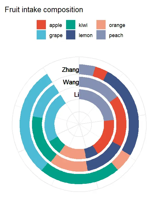
代码解释

输入数据前6行

   name label  group    percent
1 Zhang Zhang  peach 0.04796806
2 Zhang Zhang  apple 0.03954505
3 Zhang Zhang  lemon 0.28272898
4 Zhang Zhang orange 0.05662262
5 Zhang Zhang   kiwi 0.24342806
6 Zhang Zhang  grape 0.32970722

---

加载包

library(ggsci)
library(ggplot2)
library(purrr)
library(dplyr)
library(openxlsx)

读入数据

data <- read.csv("example.csv")
#下列为关键一步，产生画图需要的坐标信息
data2 <- data %>% group_by(name) %>% mutate(ymax=cumsum(percent),
                                            ymin=cumsum(percent)-percent,
                                            xmax = 0.8 + (as.numeric(cur_group_id())),
                                            xmin= (as.numeric(cur_group_id())),
                                            label_pos=(xmax+xmin)/2)%>% ungroup()
 
dfs <- split.data.frame(data2, data2$name) #将数据框拆分为列表，每个列表代表一个环

画图

#采用循环的方式生成每层的环
p_circle=lapply(dfs, function(x) {
    p1 <- geom_rect(data=x, aes(ymax=ymax, ymin=ymin, xmax=xmax, xmin=xmin, fill=group))
    p1 }
)
#采用循环的方式生成每层的标签
p_text=lapply(dfs, function(x) {
    p1 <- geom_text(data=x, aes(y=0, x=label_pos, label= label), angle=0, hjust=1)
    p1 }
)
 
#对应每层的环和标签
all_layers <- c(p_circle, p_text)
#选择配色数量
num <- data2$group %>% unique() %>% length()
#使用purrr包的reduece函数绘制所有图层
p <- reduce(all_layers, `+`, .init = ggplot())+
    coord_polar(theta = "y")+
    ylim(0, 1.1)+xlim(-1, NA)+theme_minimal()+
    theme(legend.position = "top")+
    scale_fill_manual(values=ggsci::pal_npg()(num))+
    theme(axis.text=element_blank())+labs(x=NULL,y=NULL, fill=NULL)+ggtitle("Fruit intake composition")
p
绘图
ggsave("example.png", p, height=7, width=7, bg="white")

所有代码

library(ggsci)
library(ggplot2)
library(purrr)
library(dplyr)
library(openxlsx)
 
#加载数据
data <- read.csv("example.csv")
data2 <- data %>% group_by(name) %>% mutate(ymax=cumsum(percent),
                                            ymin=cumsum(percent)-percent,
                                            xmax = 0.8 + (as.numeric(cur_group_id())),
                                            xmin= (as.numeric(cur_group_id())),
                                            label_pos=(xmax+xmin)/2)%>% ungroup()
 
dfs <- split.data.frame(data2, data2$name)
#可视化
p_circle=lapply(dfs, function(x) {
    p1 <- geom_rect(data=x, aes(ymax=ymax, ymin=ymin, xmax=xmax, xmin=xmin, fill=group))
    p1 }
)
 
p_text=lapply(dfs, function(x) {
    p1 <- geom_text(data=x, aes(y=0, x=label_pos, label= label), angle=0, hjust=1)
    p1 }
)
 
all_layers <- c(p_circle, p_text)
 
num <- data2$group %>% unique() %>% length()
 
p <- reduce(all_layers, `+`, .init = ggplot())+
    coord_polar(theta = "y")+
    ylim(0, 1.1)+xlim(-1, NA)+theme_minimal()+
    theme(legend.position = "top")+
    scale_fill_manual(values=ggsci::pal_npg()(num))+
    theme(axis.text=element_blank())+labs(x=NULL,y=NULL, fill=NULL)+ggtitle("Fruit intake composition")
p
ggsave("example.png", p, height=7, width=7, bg="white")
#版本信息
sessionInfo()